Shock analyses#

This workflow covers the standard way to apply a shock to a database by creating a new scenario via the dedicate Excel template.

Core methods#

The two main entry points are:

Database.get_shock_excel to write the workbook template;
Database.shock_calc to read that workbook and store a shocked scenario.

Typical flow#

The usual sequence is:

generate a template workbook from the current database
fill the rows you want to shock
apply the workbook into a named scenario

Apply shocks to IOTs#

Load the test IOT table embedded into MARIO

[1]:

import mario
db_IOT = mario.load_test("IOT")

INFO Parser: excel reading IOT flows from /Users/lorenzorinaldi/Documents/GitHub/MARIO/mario/test/tables/test_IOT_standard.xlsx.
INFO Parser: state payload ready with 6 canonical blocks.
INFO Parser: excel state ready for IOT.
INFO Metadata: initialized.

Generate an empty shock template#

[ ]:

db_IOT.get_shock_excel(
    path="/path/to/shock_IOT_template.xlsx",
)

Fill shock template#

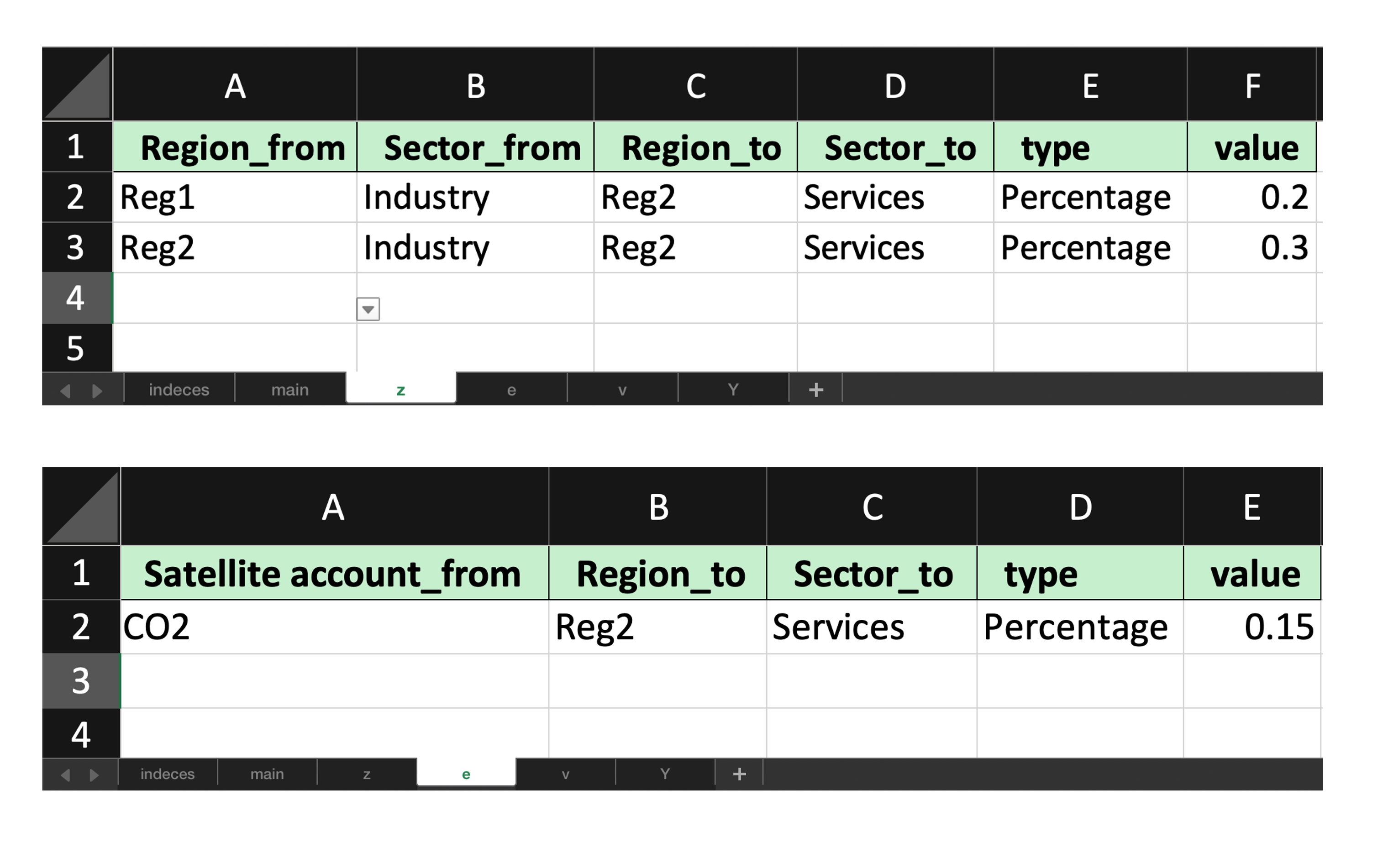
Fill the shocked template to simulate a change in consumption of “Industry” outputs from both “Reg1” and “Reg2” by “Services” sector in “Reg2”, which would cause also an increase in CO2 emissions of such sector.

These changes affect only z and e matrices

Being a simplified example, only “Percentage” change type are adopted, but also “Absolute” and “Update” changes could be used

shock_iot_template

Apply a filled shock workbook#

For IOTs, the matrices that can be shocked are z, v, e and Y.

In our example, the filled workbook updates one z and e coefficient matrices. We use the scenario argument to define the output name of the new scenario. If omitted, MARIO creates a name such as shock 1 automatically.

Download the packaged example workbooks#

The exact workbooks used in this notebook are available here:

[ ]:

db_IOT.shock_calc(
    io="/path/to/shock_IOT_filled.xlsx",
    z=True,
    e=True,
    scenario="example shock",
)

INFO Resolver: resolving z for baseline.
INFO Resolver: trying z via formula build_iot_z_from_Z_X.
INFO Resolver: resolved z via formula build_iot_z_from_Z_X.
INFO Resolver: resolving X for baseline.
INFO Resolver: trying X via formula build_iot_X_from_Z_Y.
INFO Resolver: resolved X via formula build_iot_X_from_Z_Y.
INFO Resolver: resolving e for baseline.
INFO Resolver: trying e via formula build_iot_e_from_E_X.
INFO Resolver: resolved e via formula build_iot_e_from_E_X.
INFO Resolver: resolving v for baseline.
INFO Resolver: trying v via formula build_iot_v_from_V_X.
INFO Resolver: resolved v via formula build_iot_v_from_V_X.
INFO Shock: Shock implemented successfully.

You will notice the database now has 2 scenarios

[7]:

db_IOT.scenarios

[7]:

['baseline', 'example shock']

Inspect the shocked coefficient matrix#

The query method can also be used to check variations (absolute or relative) of matrices across scenarios.

[8]:

db_IOT.query(
    matrices="z",
    scenarios="example shock",
    base_scenario="baseline",
    type="relative"
)

[8]:

		Region	Reg1			Reg2
		Level	Sector			Sector
		Item	Agriculture	Industry	Services	Agriculture	Industry	Services
Region	Level	Item
Reg1	Sector	Agriculture	0.0	0.0	0.0	0.0	0.0	0.0
		Industry	0.0	0.0	0.0	0.0	0.0	0.2
		Services	0.0	0.0	0.0	0.0	0.0	0.0
Reg2	Sector	Agriculture	0.0	0.0	0.0	0.0	0.0	0.0
		Industry	0.0	0.0	0.0	0.0	0.0	0.3
		Services	0.0	0.0	0.0	0.0	0.0	0.0

query(...) is still the most direct way to inspect exact coefficients. When you want a faster visual scan of where the shock is concentrated, you can use plot(...) on the same matrix.

The first plot below shows the relative variation of the shocked scenario against the baseline.

[10]:

db_IOT.plot(
    matrix="Z",
    scenarios=["example shock"],
    base_scenario="baseline",
    difference="relative",
    preset="heatmap",
    auto_open=False,
    path=False,
)

You can also compare the raw matrix values side by side across scenarios, for example by faceting on Scenario.

[11]:

db_IOT.plot(
    matrix="Z",
    scenarios=["baseline", "example shock"],
    preset=None,
    kind="bar",
    x="Sector_from",
    color="Sector_to",
    facet_col="Scenario",
    filters={"Region_from": ["Reg1"], "Region_to": ["Reg1"]},
    top_n=6,
    auto_open=False,
    path=False,
)

Apply shocks to SUTs#

Load the test SUT table embedded into MARIO

[13]:

import mario
db_SUT = mario.load_test("SUT")

INFO Parser: excel reading SUT flows from /Users/lorenzorinaldi/Documents/GitHub/MARIO/mario/test/tables/test_SUT_standard.xlsx.
INFO Parser: state payload ready with 10 canonical blocks.
INFO Parser: excel state ready for SUT.
INFO Metadata: initialized.

Generate an empty shock template#

[ ]:

db_SUT.get_shock_excel(
    path="/path/to/shock_SUT_template.xlsx",
)

Fill shock template#

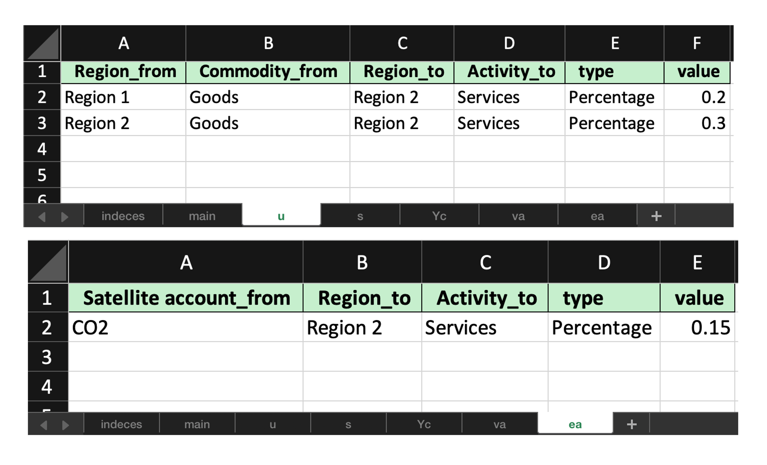
To simulate a similar shock with respect to the IOT case, fill the shock template to simulate a change in consumption of “Goods” outputs from both “Region 1” and “Region 2” by “Services” activity in “Region 2”, which would cause also an increase in CO2 emissions of such sector.

These changes affect now the u (instead of z) and ea (instead of e) matrices.

Again, only “Percentage” change type are adopted.

shock_sut_template

Apply a filled shock workbook#

For SUTs, the matrices that can be shocked are:

u and s instead of z
va and vc instead of v
ea and ec instead of e
Ya and Yc instead of Y

In our example, the filled workbook updates one u and ea coefficient matrices.

N.B. The template workbook will only generate non-fully empty matrices (e.g. in this example ec is fully empty)

[ ]:

db_SUT.shock_calc(
    io="/path/to/shock_SUT_filled.xlsx",
    z=True,
    e=True,
    scenario="example shock",
)

INFO Resolver: resolving Y for baseline.
INFO Resolver: trying Y via concat.
INFO Resolver: resolved Y via concat.
INFO Resolver: resolving Xa for baseline.
INFO Resolver: trying Xa via formula build_sut_Xa_from_S_Ya.
INFO Resolver: resolved Xa via formula build_sut_Xa_from_S_Ya.
INFO Resolver: resolving Xc for baseline.
INFO Resolver: trying Xc via formula build_sut_Xc_from_U_Yc.
INFO Resolver: resolved Xc via formula build_sut_Xc_from_U_Yc.
INFO Resolver: resolving v for baseline.
INFO Resolver: trying v via concat.
INFO Resolver: resolved v via concat.
INFO Shock: Shock implemented successfully.

[17]:

db_SUT.scenarios

[17]:

['baseline', 'example shock']

Inspect the shocked coefficient matrix#

Use again the query method

[18]:

db_SUT.query(
    matrices="u",
    scenarios="example shock",
    base_scenario="baseline",
    type="relative"
)

INFO Resolver: resolving u for example shock.
INFO Resolver: trying u via extract.
INFO Resolver: resolved u via extract.

[18]:

		Region	Region 1		Region 2
		Level	Activity		Activity
		Item	Manufacturing	Services	Manufacturing	Services
Region	Level	Item
Region 1	Commodity	Goods	0.0	0.0	0.0	0.2
Region 1	Commodity	Services	0.0	0.0	0.0	0.0
Region 2	Commodity	Goods	0.0	0.0	0.0	0.3
Region 2	Commodity	Services	0.0	0.0	0.0	0.0

Again, keep query(...) as the standard workflow when you need the exact numbers. plot(...) is useful as a complementary step to identify patterns and hotspots before drilling back into the table.

This example visualizes the relative change in the shocked u matrix compared with the baseline.

[19]:

db_SUT.plot(
    matrix="U",
    scenarios=["example shock"],
    base_scenario="baseline",
    difference="relative",
    preset="heatmap",
    auto_open=False,
    path=False,
)

INFO Resolver: resolving U for example shock.
INFO Resolver: trying U via extract.
INFO Resolver: resolved U via extract.

If you prefer to inspect absolute values instead of differences, plot both scenarios together and facet the result by Scenario.

[22]:

db_SUT.plot(
    matrix="U",
    scenarios=["baseline", "example shock"],
    preset=None,
    kind="bar",
    x="Commodity_from",
    color="Activity_to",
    facet_col="Scenario",
    filters={"Region_from": ["Region 1"], "Region_to": ["Region 1"]},
    top_n=6,
    auto_open=False,
    path=False,
)

Clusters#

Shock templates and shock application both understand clusters.

You can:

rely on default clusters already available on the database (e.g. “all” for Regions)
store reusable custom clusters on the database
pass ad hoc clusters directly to get_shock_excel(...) or shock_calc(...)

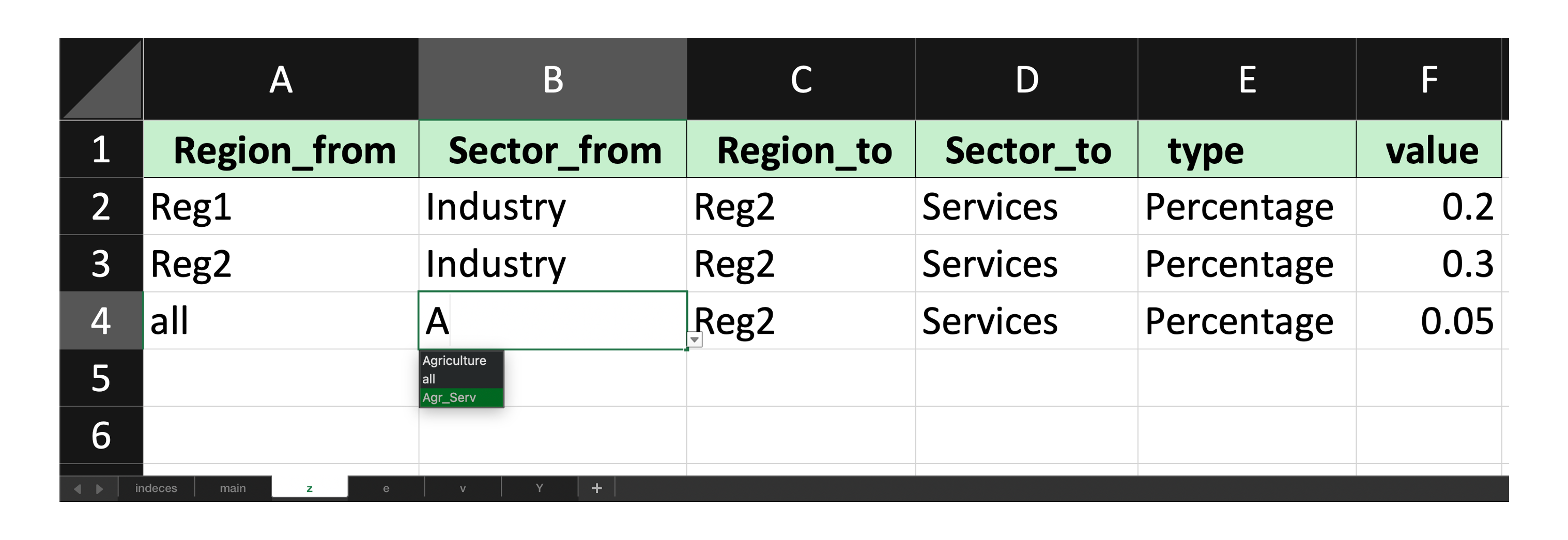
This is useful when a single workbook row should target multiple regions, sectors, activities, commodities, or final-demand categories at once.

[23]:

clusters = {
    'Sector': {
        'Agr_Serv': ['Agriculture', 'Services']
    }
}

[ ]:

db_IOT.get_shock_excel(
    path="/path/to/shock_IOT_template_clusters.xlsx",
    clusters=clusters
)

When passing the clusters argument, you will see the clusters are allowed to be selected.

shock_iot_clusters

Then with the shock_calc method, you can parse the template back.

[ ]:

db_IOT.shock_calc(
    io="/path/to/shock_IOT_filled_clusters.xlsx",
    z=True,
    e=True,
    scenario="example shock clusters",
    clusters=clusters
)

INFO Shock: Shock implemented successfully.

[27]:

db_IOT.query(
    matrices="Z",
    scenarios="example shock clusters",
    base_scenario="example shock",
    type="relative"
)

[27]:

		Region	Reg1			Reg2
		Level	Sector			Sector
		Item	Agriculture	Industry	Services	Agriculture	Industry	Services
Region	Level	Item
Reg1	Sector	Agriculture	0.000179	0.000087	0.000077	0.009694	0.005164	0.074003
		Industry	0.000179	0.000087	0.000077	0.009694	0.005164	0.022860
		Services	0.000179	0.000087	0.000077	0.009694	0.005164	0.074003
Reg2	Sector	Agriculture	0.000179	0.000087	0.000077	0.009694	0.005164	0.074003
		Industry	0.000179	0.000087	0.000077	0.009694	0.005164	0.022860
		Services	0.000179	0.000087	0.000077	0.009694	0.005164	0.074003

Download this notebook