Structural path analysis#
This notebook shows how to use db.calc_spa(...) on EXIOBASE with MARIO.
The case study focuses on the CO2 footprint of German final demand for motor vehicles in 2022. The target sector and indicator are fixed explicitly, so the notebook can focus on selecting and expanding one German final-demand bundle.
[1]:
import mario

mario.set_palette("mario")
1. Configure the case study#
We reuse the same local EXIOBASE folder as the supply-chain notebook, but now the analytical question is narrower: which upstream paths dominate the CO2 footprint of German final demand for motor vehicles in 2022?
[2]:
FOLDER = r"/Users/lorenzorinaldi/Library/CloudStorage/OneDrive-SharedLibraries-PolitecnicodiMilano/DENG-SESAM - Documenti/c-Research/a-Datasets/_Input Output Databases/EXIOBASE/3.10.1"
TABLE = "IOT"
YEAR = 2022
SYSTEM = "pxp"
SECTOR = "Motor vehicles, trailers and semi-trailers (34)"
INDICATOR = "CO2 - combustion - air"
TARGET_REGION = "DE"
BUNDLE_RANK = 0
MAX_DEPTH = 10
CUTOFF_SHARE = 0.001
TOP_N = 20
2. Parse one EXIOBASE year#
One year is enough for one SPA run. After parsing, the database contains the matrices needed to identify the focal sector, select one final-demand bundle, and expand the dominant upstream paths.
[3]:
db = mario.parse_exiobase(
    path=f"{FOLDER}/{TABLE}_{YEAR}_{SYSTEM}.zip",
    table="IOT",
    unit="Monetary",
)
db
INFO Parser: reading EXIOBASE IOT from /var/folders/7_/vg3_ld6n2pd73xyzt9dcdhlc0000gn/T/mario_exiobase_iot_zx6d1uct.
INFO Parser: reading EXIOBASE IOT extensions from /var/folders/7_/vg3_ld6n2pd73xyzt9dcdhlc0000gn/T/mario_exiobase_iot_zx6d1uct.
INFO Parser: using split extension layout with 7 extension directories.
INFO Parser: EXIOBASE IOT parsed with 200 sectors, 9 value-added rows and 725 extension rows.
INFO Metadata: initialized.
[3]:
name = EXIO_IOT_2022_pxp
table = IOT
scenarios = ['baseline']
Factor of production = 9
Satellite account = 725
Consumption category = 7
Region = 49
Sector = 200
3. Fixed target#
The target sector and indicator are set directly in the configuration cell above, so no extra label-resolution step is needed in the workflow.
4. Inspect German final demand for the focal sector#
Before running SPA, it helps to see where the focal motor-vehicle sector is sold directly inside German final demand. The notebook ranks the German destination bundles and uses the largest one as the focal demand bundle for the next step.
[4]:
direct_final_demand = (
    db.Y.loc[(slice(None), slice(None), SECTOR), :]
    .loc[:, lambda frame: frame.columns.get_level_values(0) == TARGET_REGION]
    .sum(axis=0)
    .sort_values(ascending=False)
    .rename("Direct final demand")
)
direct_final_demand = direct_final_demand[direct_final_demand != 0]
direct_final_demand.head(10)
[4]:
Region  Level                 Item
DE      Consumption category  Final consumption expenditure by households    154583.411697
                              Gross fixed capital formation                   59998.089082
                              Changes in inventories                          -5815.191944
Name: Direct final demand, dtype: float64
[5]:
if direct_final_demand.empty:
    raise ValueError(f"No direct final demand was found for {SECTOR} in {TARGET_REGION}.")
focus_bundle = direct_final_demand.index[BUNDLE_RANK]
FOCUS_REGION = focus_bundle[0]
FOCUS_CATEGORY = focus_bundle[-1]
selected_bundle_demand = db.Y.loc[
    (slice(None), slice(None), SECTOR),
    focus_bundle,
]
selected_bundle_demand = selected_bundle_demand[selected_bundle_demand != 0]
total_footprint = sum(
    float(db.f.loc[INDICATOR, node]) * float(value)
    for node, value in selected_bundle_demand.items()
)
CUTOFF = abs(total_footprint) * CUTOFF_SHARE
{
    "Sector": SECTOR,
    "Indicator": INDICATOR,
    "Region": FOCUS_REGION,
    "Category": FOCUS_CATEGORY,
    "Direct final demand": float(direct_final_demand.iloc[BUNDLE_RANK]),
    "Total footprint": total_footprint,
    "Cutoff": CUTOFF,
}
INFO Resolver: resolving f for baseline.
INFO Resolver: trying f via formula build_iot_f_from_e_w (compute_method=auto, runtime=inverse).
INFO Resolver: resolved f via formula build_iot_f_from_e_w (compute_method=auto, runtime=inverse).
[5]:
{'Sector': 'Motor vehicles, trailers and semi-trailers (34)',
 'Indicator': 'CO2 - combustion - air',
 'Region': 'DE',
 'Category': 'Final consumption expenditure by households',
 'Direct final demand': 154583.4116965654,
 'Total footprint': 37657332602.54765,
 'Cutoff': 37657332.60254765}
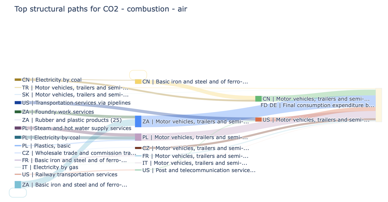
5. Run structural path analysis with MARIO#
db.calc_spa(...) renders the built-in SPA view directly inside the notebook. Here the main chart is the integrated plot="sankey" view, so MARIO displays the dominant structural paths for the selected German final-demand bundle as a network while still returning the ranked path table below.
[14]:
spa = db.calc_spa(
    indicator=INDICATOR,
    scenario="baseline",
    item=SECTOR,
    final_demand_region=FOCUS_REGION,
    final_demand_category=FOCUS_CATEGORY,
    max_depth=MAX_DEPTH,
    cutoff=CUTOFF,
    top_n=TOP_N,
    plot="sankey",
    show_plot=False,
    title=f"Top structural paths for {INDICATOR}",
)
[13]:
spa.attrs
[13]:
{'indicator': 'CO2 - combustion - air',
 'scenario': 'baseline',
 'item': 'Motor vehicles, trailers and semi-trailers (34)',
 'unit': 'kg',
 'total_footprint': 37657332602.54765,
 'reported_contribution': 5192567349.419048,
 'coverage_share': 0.13788994043268354,
 'max_depth': 10,
 'cutoff': 37657332.60254765}
6. Summarize the path structure by depth#
After the Sankey overview, a second MARIO-native read is by upstream depth. This section uses the integrated plot="depth" view of db.calc_spa(...) and removes the top_n cap, so the summary reflects all paths that survive the cutoff rather than only the ranked Sankey subset.
[8]:
spa_full = db.calc_spa(
    indicator=INDICATOR,
    scenario="baseline",
    item=SECTOR,
    final_demand_region=FOCUS_REGION,
    final_demand_category=FOCUS_CATEGORY,
    max_depth=MAX_DEPTH,
    cutoff=CUTOFF,
    top_n=None,
    plot="depth",
    show_plot=True,
    title=f"Footprint by SPA depth for {INDICATOR}",
)
The same pattern can be reused with another indicator, another sector, or another EXIOBASE year. For this German motor-vehicles example, the most useful next variations are usually: comparing household versus investment demand, testing another manufacturing sector, or checking how the dominant CO2 paths shift over time.